Overview
Behaviour Over Convenience: Modelling Scenario Risks in QCRA
Many project risks do not behave like a smooth range. They either do not occur at all, or they occur and land in one of a few discrete outcomes. Yet, we routinely force these scenario-style risks into three-point estimates because the template expects it. That is not simplification, it is a distortion of behaviour, especially in the tail where P90 decisions are made.
This is the 3rd article in a short series on modelling uncertainty based on how risks actually behave in complex projects.
Related reading (optional):
Article 1: Better Than Rules of Thumb, Choosing Risk Distributions by Testing Behaviour, Not Opinion
Article 2: Advanced Risk Modelling in @Risk: Behaviour-Driven Patterns for QCRA
Behaviour first
Before choosing any distribution, ask:Does this risk behave like a smooth range, or a set of outcomes?
Many project risks behave like outcomes, not ranges. For example:
Design: minor comments requiring limited rework, moderate comments requiring partial redesign, full redesign, or late scope change and re-approval.
Procurement: small premium, re-tendering, a changed supplier strategy, or higher-cost supply chain.
Scope growth: one scope item, multiple scope items, or a change large enough to invalidate the current baseline.
These are scenario sets. The modelling approach should reflect that.
The pattern that matches scenario risks
Once you recognise a scenario-style risk, the modelling pattern is straightforward:
Does the event occur at all?
If it occurs, which outcome materialises?
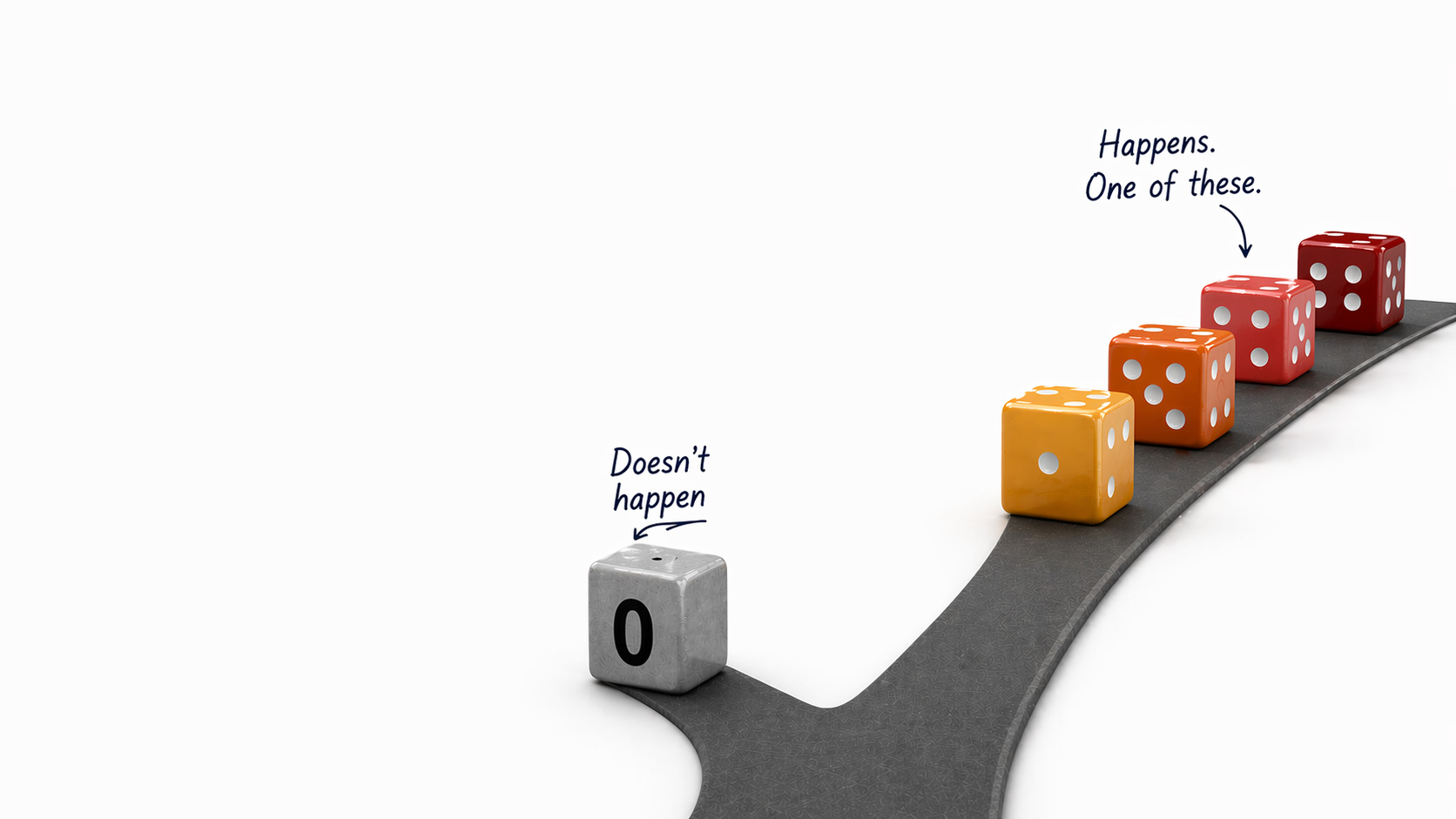
Total impact is either $0 or one of the defined scenario impacts.
This is two layers:
Occurrence (does the event happen), and
Consequence (which outcome occurs if it does).
Key rule:
Apply the occurrence probability once, then let scenario logic determine the realised impact. For scenario risks, $0 belongs to non-occurrence. Once the risk occurs, the minimum consequence should represent the least-impactful credible outcome, unless some scenarios affect other objectives but not cost.
Example you can lift straight into a model
Risk: Scope growth late in designleads to rework, cost escalation, and delays
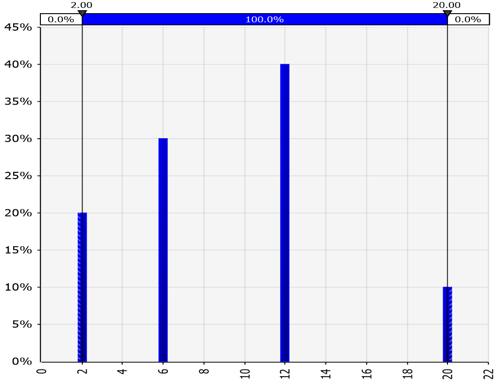
Occurrence likelihood (p): 40%
If it occurs, there are four mutually exclusive outcomes:
Scenario A (20%): Scope Item 1 only, limited interface impact, $2m
Scenario B (30%): Scope Item 2 only, higher complexity, $6m
Scenario C (40%): Items 1 and 2, rework and interfaces, $12m
Scenario D (10%): Items 1 and 2 plus re-baseline and knock-ons, $20m
Correct behaviour in the simulation:
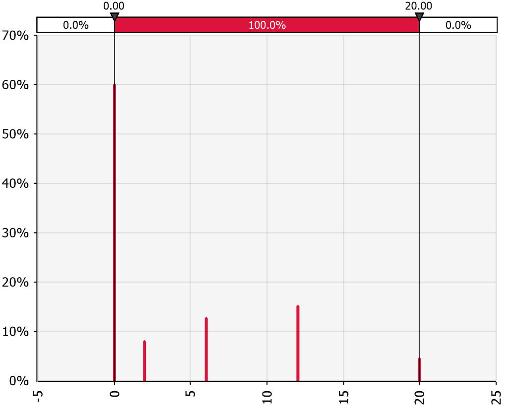
60% of iterations: $0
40% of iterations: exactly one of $2m, $6m, $12m, $20m, selected in line with the scenario weights.
That spike at zero plus occasional large jumps is the point (see Figure 1 and Figure 2). It disappears when you replace this with a single averaged input.
Route 1: You can edit the QCRA model (cleanest)
Occurrence cell (0 or 1)Use any standard binary event function such as:RiskBernoulli(p) or RiskBinomial(1,p) or RiskDiscrete({0,1},{1-p,p})Scenario impact cell (one outcome per iteration)Use a discrete selector to ensure exactly one scenario is chosen per iteration. For example: RiskDiscrete({2,6,12,20},{20%,30%,40%,10%})
Calculated impact cellImpact = Occurrence × ScenarioImpact
Link output into aggregationEnsure the resulting impact feeds into the total risk exposure calculation.
Discrete is often the clearest way to do thisin most risk modelling tools, but the key requirement is that the model selects exactly one scenario outcome per iteration, rather than spreading impact across a smooth range.
This keeps review simple: probability is applied once, outcomes stay discrete, and behaviour can be checked directly.
Route 2: You are constrained by a QCRA model or RMIS export
If bespoke logic is hard to add, you still have better options than averaging the risk into one number.
Option 2A: Split into separate risk lines (with an exclusivity note)
Use this option when you cannot embed scenario logic in the QCRA model, but you can still add or modify risk lines.This is not as robust as embedding true scenario logic in the model, but it is preferable to collapsing the risk into a single EMV value.
Turn the one underlying risk into multiple scenario risks, each representing an alternative outcome of the same parent risk.
For SG-01 (Late design scope growth):
Risk SG-01ALikelihood = 40% × 20% = 8%Impact = $2m
Risk SG-01BLikelihood = 40% × 30% = 12%Impact = $6m
Risk SG-01CLikelihood = 40% × 40% = 16%Impact = $12m
Risk SG-01DLikelihood = 40% × 10% = 4%Impact = $20m
Use a controlled and consistent naming convention so it is clear these are alternative scenario outcomes of a single underlying risk, for example SG-01A, SG-01B, SG-01C, SG-01D, all explicitly linked back to the parent risk SG-01 in the risk ID, description, or notes field.
Limitation:
Option 2A is acceptable as a workaround, but it is not behaviourally equivalent to a true scenario model.The QCRA model may not enforce mutual exclusivity, so tail behaviour can be distorted. Avoid relying on this for tail-sensitive decisions unless supported by companion scenario runs (Option 2D).
Option 2B: Mapping layer outside QCRA model
When to use itRMIS and the QCRA model are locked, but you can add a controlled mapping step between them.
What this looks like
RMIS holds one parent risk ID (SG-01).
An Excel mapping table sits outside the QCRA model and converts the RMIS export into model-ready scenario inputs.
The QCRA model reads the mapped output during the simulation.
How it works in practice
SG-01 stays as one risk in RMIS.
The mapping expands it into:
occurrence probability (p),
scenario probabilities (for example 20%,30%,40%,10%),
scenario impacts (for example $2m, $6m, $12m, $20m).
The mapping layer generates one scenario-consistent impact value per iteration, consistent with the logic set out in Route 1.
That single simulated impact value is then linked into the QCRA model's total risk calculation, just like any other risk input.
Option 2C: Local scenario block inside the QCRA model
When to use itThe RMIS and corporate QCRA template are fixed, but you are permitted to add a small local block within the QCRA model and link one cell into the total risk calculation.
What this looks like
A compact block for SG-01 that implements:
occurrence logic (for example RiskBernoulli(40)),
mutually exclusive scenario selection (for example RiskDiscrete({2,6,12,20},{20%,30%,40%,10%})),
calculated impact (Occurrence × ScenarioImpact).
One calculated impact cell referenced by the SG-01 line item, so the total risk calculation uses the scenario block instead of a single averaged input.
LimitationUse selectively. Too many bespoke blocks make the model harder to maintain and review.
Key distinction, now implicit in the text
2B keeps scenario logic outside the QCRA model to satisfy governance constraints, with the model reading a mapped value during the simulation.
2C implements the same logic within the QCRA file, where the coremodel structure is fixed but controlled additions are still permitted.
Important:
Where occurrence and scenario logic are implemented via Option 2B or 2C, the SG-01 line item in the QCRA total should function as a 100% pass-through, with no additional likelihood applied.
For Option 2B and 2C, wrap the final scenario-consistent impact cell in RiskMakeInput() so it is treated as a primary input distribution, allowing the total risk tornado and sensitivity outputs to operate properly. Apply this to the final calculated impact, not to the individual components.
Option 2D: Companion scenario runs (sensitivity view)
Use when the model is locked and cannot represent scenario logic, but you still need to see tail sensitivity. This is not probabilistic modelling, it is controlled sensitivity analysis alongside the official model.
For SG-01:
Reference case: force SG-01 to $0, record P90_Base.
Stress cases:run separate simulations forcing SG-01 to each scenario impact in turn, $2m, $6m, $12m, $20m, and record the resulting P90 for each run.
Interpretation: compare to P90_Base. Deltas show how each realised scenario shifts the tail, without averaging or inventing a smooth distribution.
The conditional weighting between scenarios is not modelled here. Each scenario is tested independently to assess its impact on the tail. Present this as governance insight, not as a substitute for scenario-based probabilistic modelling.
Which option should I use?
If the risk materially affects P80 to P95, avoid 2A unless supported by 2D.
If governance allows an external mapping step, prefer 2B.
If you can embed local logic inside the QCRA model, prefer 2C.
If nothing can change, use 2D for transparency and sensitivity insight, not for calibration.
Note: Forcing risks on and off is a simple way to confirm the workaround behaves as intended.
The three traps that quietly break scenario modelling
Trap 1: Replacing a scenario risk with an "average" value
People take several discrete outcomes, calculate an average (or EMV), and feed that single number into the simulation. It feels tidy, but it collapses the distribution. You lose the spike at zero and the lumpy jumps that drive P90. For scenario risks, a single smooth input is not simplification, it is deletion.
Trap 2: Applying probability twice
If occurrence is already modelled via a 0 or 1 event, probability has already been applied. Applying p again elsewhere quietly shrinks impacts and understates tails. A common symptom is that the simulated mean drops below the expected value without a clear behavioural reason.Occurrence probability should live in one place only.
Trap 3: Forcing a smooth 3-point distribution because a template expects it
PERT and triangular work when a risk behaves like a continuous range. If a risk has discrete outcomes, blocky jumps, or threshold behaviour, a smooth curve can create impacts that never occur and still understate rare but severe outcomes. The issue is behaviour, the model should reflect how the risk actually manifests, not what a template happens to accept.
Where distributions fit in, without getting lost in the menu
The purpose of this section is not to encourage more complex modelling. It is to make the available tools understandable. Many of these distributions appear in risk modelling software, and practitioners often encounter them without clear guidance on when, or whether, they should be used.
In most cases, simpler structures that reflect behaviour clearly are preferable to more complex ones that are harder to explain and review. The goal is not to use more distributions, but to use the simplest approach that is behaviourally correct, transparent, and defensible.
The examples below use @Risk function names purely for illustration, as they are widely recognised by practitioners. Other risk modelling tools offer equivalent distributions and functionality, and the underlying concepts remain the same.
Discrete, when outcomes are genuinely discreteUse this when there are a small number of clearly defined outcomes with no meaningful values in between. This aligns with scenario-style risks, where impact occurs as one of several distinct outcomes if the risk materialises (see Figure 1).
Examples:
Rail possession disruption: loss of one planned weekend possession, loss of two consecutive weekend possessions, requirement for an additional major possession window.
Design review risk: minor comments requiring limited rework, partial redesign of affected elements, full redesign, late scope change following redesign.
Approval risk: approval granted with conditions requiring rework, rejection requiring resubmission, or prolonged review that delays downstream activities.
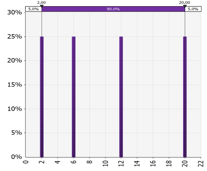
DUniform, when outcomes are discrete and genuinely equal likelihoodThis is the uniform distribution in discrete mode, meaning it selects one value from a set of discrete outcomes with equal chance (see Figure 3).Function: RiskDUniform({2,6,12,20})
Examples:
Early procurement strategy: multiple delivery options are credible and you genuinely cannot weight them yet.
Early concept design: several feasible solutions exist before you have enough evidence to favour one.
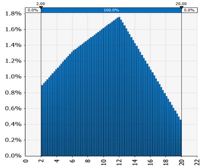
General, when you have multiple credible anchor scenarios and want a controlled rangeUse this when the risk behaves like a range and you can describe that rangeusing more than three credible anchor points. This is not a discrete distribution. It is a continuous alternative to PERT or triangular when you have more than three credible inputs, for example four or more scenarios that define the shape of the range. Each point should represent a plausible scenario, not an abstract or drawn shape (see Figure 4).Function: RiskGeneral(2,20,{2,6,12,20},{20%,30%,40%,10%})
Examples:
Progressive design developmentwhere cost impact increases with scope refinement. Instead of a three-point estimate, multiple credible cost anchors are used to shape a continuous range of possible outcomes.
Quantities growth within defined scope boundaries where more than three credible quantity or cost anchors are available. Instead of a three-point estimate, these anchors are used to define a continuous range of possible outcomes.
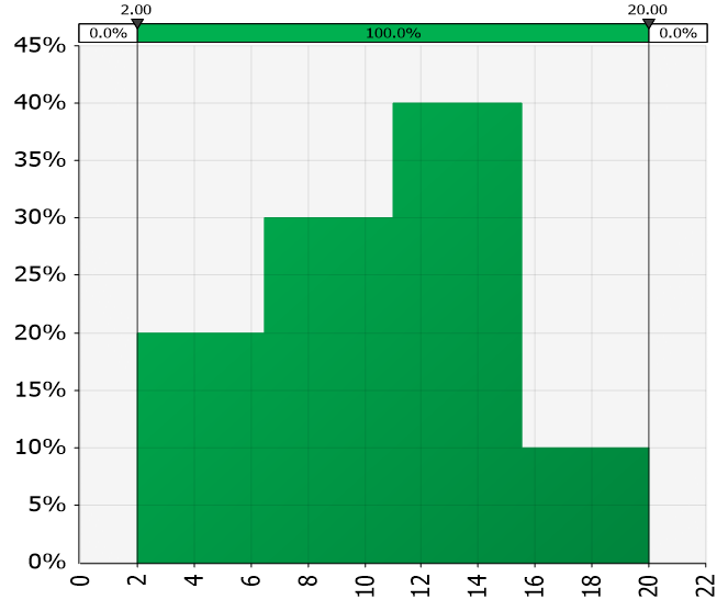
Histogram, when stakeholders think in bracketsUse this when SMEs naturally estimate impacts in brackets, and the likelihood differs by bracket (see Figure 5).Function: RiskHistogram(2,20,{20%,30%,40%,10%})
Examples:
Latent conditions or remediation, where mid-range brackets are most common but tails remain credible
Utilities relocation, where moderate outcomes dominate and a high bracket exists due to unknown services or access constraints
@Risk Artist, when you need to draw the behaviour@Risk Artist lets you draw the shape of a distribution with as many anchor points as you want, in a continuous fashion. @Risk then converts that curve into a distribution you can simulate.
Treat it as a niche tool with limited practical value in most project risk applications. It is worth being aware of, but not something you would typically use in practice.
What's next
This article focused on how to represent scenario-style risks when systems and templates are constrained, and why forcing them into three-point estimates distorts tail behaviour.
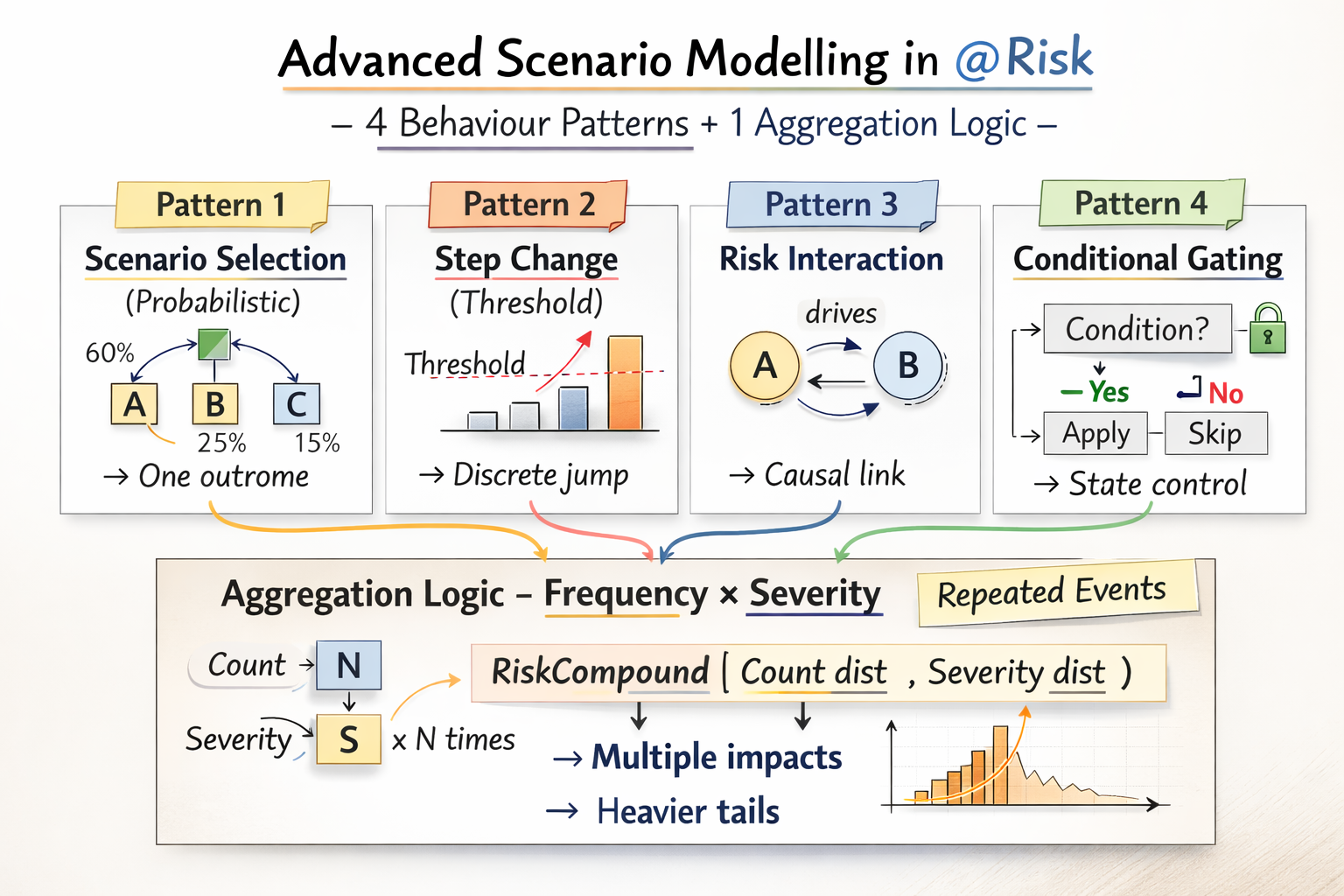
In the previous articles, I first looked at how distribution choice shapes uncertainty and tail behaviour, and then explored more advanced modelling patterns for representing conditional behaviour directly inside a QCRA model, including probabilistic scenario selection, step-change impacts, risk interaction logic, and conditional gating.
The series will now shift from modelling to quality assurance. I will look at practical approaches for reviewing QCRA models, followed by a companion piece on quality assurance for QSRA models.
https://www.linkedin.com/pulse/behaviour-over-convenience-modelling-scenario-risks-qcra-amin-jalili-dazqc/